6. Neural Networks with PyTorch
In this tutorial we will show how to create a Neural Network using the PyTorch (more usage examples of PyTorch here).
6.1. Classifying blobs
First, we need to create a neural network. We simply use PyTorch nn.Module as regular PyTorch code.
[1]:
import torch
from torch import nn

class Net(nn.Module):
    """
    Model with input size (-1, 5) for blobs dataset
    with 5 features
    """
    def __init__(self, n_features, n_classes):
        """Example network."""
        super(Net, self).__init__()
        self.fc1 = nn.Linear(n_features, 5)
        self.fc2 = nn.Linear(5, n_classes)

    def forward(self, x):
        x = torch.relu(self.fc1(x))
        x = self.fc2(x)
        return x
We will use a 5D dataset composed with 3 gaussians. We can use 4k samples for training and 1k for testing. We can divide the sets in batches so that they can be processed in small groups by the network. We use a batch size of 20.
[2]:
# experiment parameters
n_classes = 3
n_features = 2
n_samples_tr = 4000  # number of training set samples
n_samples_ts = 1000  # number of testing set samples
batch_size = 20

# dataset creation
from secml.data.loader import CDLRandom
dataset = CDLRandom(n_samples=n_samples_tr + n_samples_ts,
                    n_classes=n_classes,
                    n_features=n_features, n_redundant=0,
                    n_clusters_per_class=1,
                    class_sep=1, random_state=0).load()

# Split in training and test
from secml.data.splitter import CTrainTestSplit
splitter = CTrainTestSplit(train_size=n_samples_tr,
                           test_size=n_samples_ts,
                           random_state=0)

tr, ts = splitter.split(dataset)

# Normalize the data
from secml.ml.features.normalization import CNormalizerMinMax
nmz = CNormalizerMinMax()
tr.X = nmz.fit_transform(tr.X)
ts.X = nmz.transform(ts.X)
Now we can create an instance of the PyTorch model and then wrap it in the specific class that will link it to our library functionalities.
[3]:
# torch model creation
net = Net(n_features=n_features, n_classes=n_classes)

from torch import optim
criterion = nn.CrossEntropyLoss()
optimizer = optim.SGD(net.parameters(),
                      lr=0.01, momentum=0.9)

# wrap torch model in CClassifierPyTorch class
from secml.ml.classifiers import CClassifierPyTorch
clf = CClassifierPyTorch(model=net,
                         loss=criterion,
                         optimizer=optimizer,
                         input_shape=(n_features,))
We can simply use the loaded CDataset and pass it to the fit method. The wrapper will handle batch processing and train the network for the number of epochs specified in the wrapper constructor.
[4]:
clf.fit(tr)
[1,  2000] loss: 0.281
[1,  4000] loss: 0.116
[2,  2000] loss: 0.106
[2,  4000] loss: 0.110
[3,  2000] loss: 0.100
[3,  4000] loss: 0.106
[4,  2000] loss: 0.096
[4,  4000] loss: 0.102
[5,  2000] loss: 0.095
[5,  4000] loss: 0.101
[6,  2000] loss: 0.094
[6,  4000] loss: 0.100
[7,  2000] loss: 0.092
[7,  4000] loss: 0.098
[8,  2000] loss: 0.091
[8,  4000] loss: 0.097
[9,  2000] loss: 0.090
[9,  4000] loss: 0.095
[10,  2000] loss: 0.088
[10,  4000] loss: 0.094
[4]:
CClassifierPyTorch{'classes': CArray(3,)(dense: [0 1 2]), 'n_features': 2, 'preprocess': None, 'input_shape': (2,), 'softmax_outputs': False, 'layers': [('fc1', Linear(in_features=2, out_features=5, bias=True)), ('fc2', Linear(in_features=5, out_features=3, bias=True))], 'layer_shapes': {'fc1': (1, 5), 'fc2': (1, 3)}, 'loss': CrossEntropyLoss(), 'optimizer': SGD (
Parameter Group 0
    dampening: 0
    lr: 0.01
    momentum: 0.9
    nesterov: False
    weight_decay: 0
), 'epochs': 10, 'batch_size': 1}
Using the model in “predict” mode is just as easy. We can use the method predict defined in our wrapper, and pass in the data. We can evaluate the accuracy with the CMetric defined in our library.
[5]:
label_torch = clf.predict(ts.X, return_decision_function=False)

from secml.ml.peval.metrics import CMetric
acc_torch = CMetric.create('accuracy').performance_score(ts.Y, label_torch)

print("Model Accuracy: {}".format(acc_torch))
Model Accuracy: 0.991
7. Evasion Attacks against Neural Networks on MNIST dataset
Now we do the same thing with the MNIST dataset. We can use a convolutional neural network, but we need to take care of reshaping the input to the expected input size - in this case (-1, 1, 28, 28). We will see in the following how to use torchvision’s transforms module for this.
[6]:
class MNISTNet(nn.Module):
    """
    Model with input size (-1, 28, 28) for MNIST dataset.
    """
    def __init__(self):
        super(MNISTNet, self).__init__()
        self.conv1 = nn.Conv2d(1, 10, kernel_size=5)
        self.conv2 = nn.Conv2d(10, 20, kernel_size=5)
        self.conv2_drop = nn.Dropout2d()
        self.fc1 = nn.Linear(320, 50)
        self.fc2 = nn.Linear(50, 3)

    def forward(self, x):
        x = torch.relu(torch.max_pool2d(self.conv1(x), 2))
        x = torch.relu(torch.max_pool2d(self.conv2_drop(self.conv2(x)), 2))
        x = x.view(-1, 320)
        x = torch.relu(self.fc1(x))
        return self.fc2(x)
Now we can load MNIST dataset. Here we should take care of the conversion from 1D vector to images of shape (-1, 1, 28, 28). This is a required step, since the loader defined in our library is defined to load a ravel vector with shape (-1, 1, 784).
We can use a Lambda module of the transforms package from torchvision. The lambda we define will simply reshape the tensors to the shape expected by our network.
[7]:
n_samples_tr = 6000  # number of training set samples
n_samples_ts = 1000  # number of testing set samples

from secml.data.loader import CDataLoaderMNIST
digits = (1, 5, 9)
dataset = CDataLoaderMNIST().load('training', digits=digits)

# Split in training and test
splitter = CTrainTestSplit(train_size=n_samples_tr,
                           test_size=n_samples_ts,
                           random_state=0)
tr, ts = splitter.split(dataset)

# Normalize the data
nmz = CNormalizerMinMax()
tr.X /= 255
ts.X /= 255
Now we can use again the CClassifierPyTorch wrapper for having the model accessible with our library.
[8]:
net = MNISTNet()
criterion = nn.CrossEntropyLoss()
optimizer = optim.SGD(net.parameters(),
                      lr=0.001, momentum=0.9)

clf = CClassifierPyTorch(model=net,
                         loss=criterion,
                         optimizer=optimizer,
                         epochs=20,
                         batch_size=20,
                         input_shape=(1, 28, 28))
We fit the model in the same way as before.
[9]:
clf.fit(tr)
[9]:
CClassifierPyTorch{'classes': CArray(3,)(dense: [0 1 2]), 'n_features': 784, 'preprocess': None, 'input_shape': (1, 28, 28), 'softmax_outputs': False, 'layers': [('conv1', Conv2d(1, 10, kernel_size=(5, 5), stride=(1, 1))), ('conv2', Conv2d(10, 20, kernel_size=(5, 5), stride=(1, 1))), ('conv2_drop', Dropout2d(p=0.5, inplace=False)), ('fc1', Linear(in_features=320, out_features=50, bias=True)), ('fc2', Linear(in_features=50, out_features=3, bias=True))], 'layer_shapes': {'conv1': (1, 10, 24, 24), 'conv2': (1, 20, 8, 8), 'conv2_drop': (1, 20, 8, 8), 'fc1': (1, 50), 'fc2': (1, 3)}, 'loss': CrossEntropyLoss(), 'optimizer': SGD (
Parameter Group 0
    dampening: 0
    lr: 0.001
    momentum: 0.9
    nesterov: False
    weight_decay: 0
), 'epochs': 20, 'batch_size': 20}
And now we can check how well we can classify the digits.
[10]:
label_torch = clf.predict(ts.X, return_decision_function=False)

metric = CMetric.create('accuracy')
acc_torch = metric.performance_score(ts.Y, label_torch)

print("Model Accuracy: {}".format(acc_torch))
Model Accuracy: 0.991
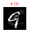
7.1. Crafting Evasion Attacks
We can now create, as we did in notebook 05-MNIST_dataset.ipynb, adversarial examples against the neural network we just trained. The code is similar to the other notebook, the only difference will be the classifier that we pass to the CAttackEvasionPGDLS object.
[11]:
# For simplicity, let's attack a subset of the test set
attack_ds = ts[:25, :]

noise_type = 'l2'  # Type of perturbation 'l1' or 'l2'
dmax = 3.  # Maximum perturbation
lb, ub = 0., 1.  # Bounds of the attack space. Can be set to `None` for unbounded
y_target = None  # None if `error-generic` or a class label for `error-specific`

# Should be chosen depending on the optimization problem
solver_params = {
    'eta': 0.3,
    'eta_min': 2.0,
    'eta_max': None,
    'max_iter': 100,
    'eps': 1e-4
}

from secml.adv.attacks import CAttackEvasionPGDLS
pgd_ls_attack = CAttackEvasionPGDLS(classifier=clf,
                                    surrogate_classifier=clf,
                                    surrogate_data=tr,
                                    distance=noise_type,
                                    dmax=dmax,
                                    solver_params=solver_params,
                                    y_target=y_target)

print("Attack started...")
eva_y_pred, _, eva_adv_ds, _ = pgd_ls_attack.run(
    attack_ds.X, attack_ds.Y, double_init=True)
print("Attack complete!")
Attack started...
Attack complete!
[12]:
acc = metric.performance_score(
    y_true=attack_ds.Y, y_pred=clf.predict(attack_ds.X))
acc_attack = metric.performance_score(
    y_true=attack_ds.Y, y_pred=eva_y_pred)

print("Accuracy on reduced test set before attack: {:.2%}".format(acc))
print("Accuracy on reduced test set after attack: {:.2%}".format(acc_attack))
Accuracy on reduced test set before attack: 76.00%
Accuracy on reduced test set after attack: 32.00%
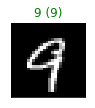
Finally, we can display the adversarial digit along with its label.
[14]:
from secml.figure import CFigure
# Let's define a convenience function to easily plot the MNIST dataset
def show_digits(samples, preds, labels, digs, n_display=8):
    samples = samples.atleast_2d()
    n_display = min(n_display, samples.shape[0])
    fig = CFigure(width=n_display*2, height=3)
    for idx in range(n_display):
        fig.subplot(2, n_display, idx+1)
        fig.sp.xticks([])
        fig.sp.yticks([])
        fig.sp.imshow(samples[idx, :].reshape((28, 28)), cmap='gray')
        fig.sp.title("{} ({})".format(digits[labels[idx].item()], digs[preds[idx].item()]),
                     color=("green" if labels[idx].item()==preds[idx].item() else "red"))
    fig.show()

show_digits(attack_ds.X[0, :], clf.predict(attack_ds.X[0, :]), attack_ds.Y[0, :], digits)
show_digits(eva_adv_ds.X[0, :], clf.predict(eva_adv_ds.X[0, :]), eva_adv_ds.Y[0, :], digits)