2.3. Poisoning Attacks against Machine Learning models¶

In this tutorial we will experiment with adversarial poisoning attacks against a Support Vector Machine (SVM) with Radial Basis Function (RBF) kernel.

Poisoning attacks are performed at train time by injecting carefully crafted samples that alter the classifier decision function so that its accuracy decreases.

As in the previous tutorials, we will first create and train the classifier, evaluating its performance in the standard scenario, i.e. not under attack. The poisoning attack will also need a validation set to verify the classifier performance during the attack, so we split the training set furtherly in two.

[1]:

random_state = 999

n_features = 2  # Number of features
n_samples = 300  # Number of samples
centers = [[-1, -1], [+1, +1]]  # Centers of the clusters
cluster_std = 0.9  # Standard deviation of the clusters

from secml.data.loader import CDLRandomBlobs
dataset = CDLRandomBlobs(n_features=n_features,
                         centers=centers,
                         cluster_std=cluster_std,
                         n_samples=n_samples,
                         random_state=random_state).load()

n_tr = 100  # Number of training set samples
n_val = 100  # Number of validation set samples
n_ts = 100  # Number of test set samples

# Split in training, validation and test
from secml.data.splitter import CTrainTestSplit
splitter = CTrainTestSplit(
    train_size=n_tr + n_val, test_size=n_ts, random_state=random_state)
tr_val, ts = splitter.split(dataset)
splitter = CTrainTestSplit(
    train_size=n_tr, test_size=n_val, random_state=random_state)
tr, val = splitter.split(dataset)

# Normalize the data
from secml.ml.features import CNormalizerMinMax
nmz = CNormalizerMinMax()
tr.X = nmz.fit_transform(tr.X)
val.X = nmz.transform(val.X)
ts.X = nmz.transform(ts.X)

# Metric to use for training and performance evaluation
from secml.ml.peval.metrics import CMetricAccuracy
metric = CMetricAccuracy()

# Creation of the multiclass classifier
from secml.ml.classifiers import CClassifierSVM
from secml.ml.kernels import CKernelRBF
clf = CClassifierSVM(kernel=CKernelRBF(gamma=10), C=1)

# We can now fit the classifier
clf.fit(tr.X, tr.Y)
print("Training of classifier complete!")

# Compute predictions on a test set
y_pred = clf.predict(ts.X)

Training of classifier complete!

2.3.1. Generation of Poisoning Samples¶

We are going to generate an adversarial example against the SVM classifier using the gradient-based algorithm for generating poisoning attacks proposed in:

[biggio12-icml] Biggio, B., Nelson, B. and Laskov, P., 2012. Poisoning attacks against support vector machines. In ICML 2012.

[biggio15-icml] Xiao, H., Biggio, B., Brown, G., Fumera, G., Eckert, C. and Roli, F., 2015. Is feature selection secure against training data poisoning?. In ICML 2015.

[demontis19-usenix] Demontis, A., Melis, M., Pintor, M., Jagielski, M., Biggio, B., Oprea, A., Nita-Rotaru, C. and Roli, F., 2019. Why Do Adversarial Attacks Transfer? Explaining Transferability of Evasion and Poisoning Attacks. In 28th Usenix Security Symposium, Santa Clara, California, USA.

To compute a poisoning point, a bi-level optimization problem has to be solved, namely:

$\begin{aligned} \max_{x_c}& A(D_{val}, \mathbf{w}^\ast) = \sum_{j=1}^m \ell(y_j, \mathbf{x_\mathit{j}}, \mathbf{w}^\ast)\\ &s.t. \mathbf{w}^\ast \in \underset{\mathbf{w}}{\operatorname{arg min}} \textit{L} (D_{tr} \cup (\mathbf{x}_c, y_c), \mathbf{w}) \end{aligned}$

Where $\mathbf{x_c}$ is the poisoning point, $A$ is the attacker objective function, $L$ is the classifier training function. Moreover, $D_{tr}$ is the validation dataset and $D_{val}$ is the training dataset. The former problem, along with the poisoning point $\mathbf{x}_c$ is used to train the classifier on the poisoned data, while the latter is used to evaluate the performance on the untainted data.

The former equation depends on the classifier weights, which in turns, depends on the poisoning point.

This attack is implemented in SecML by different subclasses of the CAttackPoisoning. For the purpose of attacking a SVM classifier we use the CAttackPoisoningSVM class.

As done for the evasion attacks, let’s specify the parameters first. We set the bounds of the attack space to the known feature space given by validation dataset. Lastly, we chose the solver parameters for this specific optimization problem.

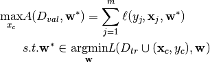
Let’s start visualizing the objective function considering a single poisoning point.

[2]:

lb, ub = val.X.min(), val.X.max()  # Bounds of the attack space. Can be set to `None` for unbounded

# Should be chosen depending on the optimization problem
solver_params = {
    'eta': 0.05,
    'eta_min': 0.05,
    'eta_max': None,
    'max_iter': 100,
    'eps': 1e-6
}

from secml.adv.attacks import CAttackPoisoningSVM
pois_attack = CAttackPoisoningSVM(classifier=clf,
                                  training_data=tr,
                                  val=val,
                                  lb=lb, ub=ub,
                                  solver_params=solver_params,
                                  random_seed=random_state)

# chose and set the initial poisoning sample features and label
xc = tr[0,:].X
yc = tr[0,:].Y
pois_attack.x0 = xc
pois_attack.xc = xc
pois_attack.yc = yc

print("Initial poisoning sample features: {:}".format(xc.ravel()))
print("Initial poisoning sample label: {:}".format(yc.item()))

from secml.figure import CFigure
# Only required for visualization in notebooks
%matplotlib inline

fig = CFigure(4,5)

grid_limits = [(lb - 0.1, ub + 0.1),
                    (lb - 0.1, ub + 0.1)]

fig.sp.plot_ds(tr)

# highlight the initial poisoning sample showing it as a star
fig.sp.plot_ds(tr[0,:], markers='*', markersize=16)

fig.sp.title('Attacker objective and gradients')
fig.sp.plot_fun(
    func=pois_attack.objective_function,
    grid_limits=grid_limits, plot_levels=False,
    n_grid_points=10, colorbar=True)

# plot the box constraint
from secml.optim.constraints import CConstraintBox
box = fbox = CConstraintBox(lb=lb, ub=ub)
fig.sp.plot_constraint(box, grid_limits=grid_limits,
                       n_grid_points=10)

fig.tight_layout()
fig.show()

Initial poisoning sample features: CArray([0.568353 0.874521])
Initial poisoning sample label: 1

../_images/tutorials_05-Poisoning_3_1.png

Now, we set the desired number of adversarial points to generate, 20 in this example.

[3]:

n_poisoning_points = 20  # Number of poisoning points to generate
pois_attack.n_points = n_poisoning_points

# Run the poisoning attack
print("Attack started...")
pois_y_pred, pois_scores, pois_ds, f_opt = pois_attack.run(ts.X, ts.Y)
print("Attack complete!")

# Evaluate the accuracy of the original classifier
acc = metric.performance_score(y_true=ts.Y, y_pred=y_pred)
# Evaluate the accuracy after the poisoning attack
pois_acc = metric.performance_score(y_true=ts.Y, y_pred=pois_y_pred)

print("Original accuracy on test set: {:.2%}".format(acc))
print("Accuracy after attack on test set: {:.2%}".format(pois_acc))

Attack started...
Attack complete!
Original accuracy on test set: 94.00%
Accuracy after attack on test set: 88.00%

We can see that the classifiers has been successfully attacked. To increase the attack power, more poisoning points can be crafted, at the expense of a much slower optimization process.

Let’s now visualize the attack on a 2D plane. We need to train a copy of the original classifier on the join between the training set and the poisoning points.

[4]:

# Training of the poisoned classifier
pois_clf = clf.deepcopy()
pois_tr = tr.append(pois_ds)  # Join the training set with the poisoning points
pois_clf.fit(pois_tr.X, pois_tr.Y)

# Define common bounds for the subplots
min_limit = min(pois_tr.X.min(), ts.X.min())
max_limit = max(pois_tr.X.max(), ts.X.max())
grid_limits = [[min_limit, max_limit], [min_limit, max_limit]]

fig = CFigure(10, 10)

fig.subplot(2, 2, 1)
fig.sp.title("Original classifier (training set)")
fig.sp.plot_decision_regions(
    clf, n_grid_points=200, grid_limits=grid_limits)
fig.sp.plot_ds(tr, markersize=5)
fig.sp.grid(grid_on=False)

fig.subplot(2, 2, 2)
fig.sp.title("Poisoned classifier (training set + poisoning points)")
fig.sp.plot_decision_regions(
    pois_clf, n_grid_points=200, grid_limits=grid_limits)
fig.sp.plot_ds(tr, markersize=5)
fig.sp.plot_ds(pois_ds, markers=['*', '*'], markersize=12)
fig.sp.grid(grid_on=False)

fig.subplot(2, 2, 3)
fig.sp.title("Original classifier (test set)")
fig.sp.plot_decision_regions(
    clf, n_grid_points=200, grid_limits=grid_limits)
fig.sp.plot_ds(ts, markersize=5)
fig.sp.text(0.05, -0.25, "Accuracy on test set: {:.2%}".format(acc),
            bbox=dict(facecolor='white'))
fig.sp.grid(grid_on=False)

fig.subplot(2, 2, 4)
fig.sp.title("Poisoned classifier (test set)")
fig.sp.plot_decision_regions(
    pois_clf, n_grid_points=200, grid_limits=grid_limits)
fig.sp.plot_ds(ts, markersize=5)
fig.sp.text(0.05, -0.25, "Accuracy on test set: {:.2%}".format(pois_acc),
            bbox=dict(facecolor='white'))
fig.sp.grid(grid_on=False)

fig.show()

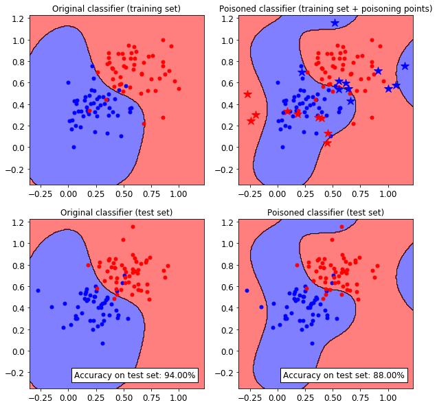
../_images/tutorials_05-Poisoning_7_0.png

We can see how the SVM classifier decision functions changes after injecting the adversarial poisoning points (blue and red stars).

For more details about poisoning adversarial attacks please refer to:

[biggio18-pr] Biggio, B. and Roli, F., 2018. Wild patterns: Ten years after the rise of adversarial machine learning. In Pattern Recognition.