1.1. Training of Classifiers and Visualization of Results
In this first tutorial we aim to show some basic functionality of SecML.
![]()
[1]:
%%capture --no-stderr --no-display
# NBVAL_IGNORE_OUTPUT

try:
  import secml
except ImportError:
  %pip install git+https://gitlab.com/secml/secml
1.1.1. Creation and visualization of a simple 2D dataset
The first step is loading the dataset. We are going to use a simple toy dataset consisting of 3 clusters of points, normally distributed.
Each dataset of SecML is a CDataset object, consisting of dataset.X and dataset.Y, where the samples and the corresponding labels are stored, respectively.
[2]:
random_state = 999

n_features = 2  # Number of features
n_samples = 1250  # Number of samples
centers = [[-2, 0], [2, -2], [2, 2]]  # Centers of the clusters
cluster_std = 0.8  # Standard deviation of the clusters

from secml.data.loader import CDLRandomBlobs
dataset = CDLRandomBlobs(n_features=n_features,
                         centers=centers,
                         cluster_std=cluster_std,
                         n_samples=n_samples,
                         random_state=random_state).load()
The dataset will be split in training and test, and normalized in the standard interval [0, 1] with a min-max normalizer.
[3]:
n_tr = 1000  # Number of training set samples
n_ts = 250  # Number of test set samples

# Split in training and test
from secml.data.splitter import CTrainTestSplit
splitter = CTrainTestSplit(
    train_size=n_tr, test_size=n_ts, random_state=random_state)
tr, ts = splitter.split(dataset)

# Normalize the data
from secml.ml.features import CNormalizerMinMax
nmz = CNormalizerMinMax()
tr.X = nmz.fit_transform(tr.X)
ts.X = nmz.transform(ts.X)
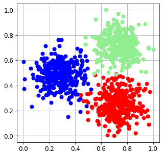
Let’s visualize the dataset in a 2D plane.
The three clusters are clearly separable and normalized as we required.
[4]:
from secml.figure import CFigure
# Only required for visualization in notebooks
%matplotlib inline

fig = CFigure(width=5, height=5)

# Convenience function for plotting a dataset
fig.sp.plot_ds(tr)

fig.show()
1.1.2. Training of classifiers
Now we can train a non-linear one-vs-all Support Vector Machine (SVM), using a Radial Basis Function (RBF) kernel for embedding.
We will evaluate the best training parameters through a 3-Fold Cross-Validation procedure, using the accuracy as the performance metric. Each classifier has an integrated routine, .estimate_parameters() which estimates the best parameters on the given training set.
[5]:
# Creation of the multiclass classifier
from secml.ml.classifiers import CClassifierSVM
from secml.ml.kernels import CKernelRBF
svm = CClassifierSVM(kernel=CKernelRBF())

# Parameters for the Cross-Validation procedure
xval_params = {'C': [0.1, 1, 10], 'kernel.gamma': [1, 10, 100]}

# Let's create a 3-Fold data splitter
from secml.data.splitter import CDataSplitterKFold
xval_splitter = CDataSplitterKFold(num_folds=3, random_state=random_state)

# Metric to use for training and performance evaluation
from secml.ml.peval.metrics import CMetricAccuracy
metric = CMetricAccuracy()

# Select and set the best training parameters for the classifier
print("Estimating the best training parameters...")
best_params = svm.estimate_parameters(
    dataset=tr,
    parameters=xval_params,
    splitter=xval_splitter,
    metric=metric,
    perf_evaluator='xval'
)

print("The best training parameters are: ",
      [(k, best_params[k]) for k in sorted(best_params)])

# We can now fit the classifier
svm.fit(tr.X, tr.Y)

# Compute predictions on a test set
y_pred = svm.predict(ts.X)

# Evaluate the accuracy of the classifier
acc = metric.performance_score(y_true=ts.Y, y_pred=y_pred)

print("Accuracy on test set: {:.2%}".format(acc))
Estimating the best training parameters...
The best training parameters are:  [('C', 1), ('kernel.gamma', 10)]
Accuracy on test set: 98.80%
1.1.3. Visualization of the decision regions of the classifiers
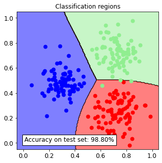
Once the classifier is trained, we can visualize the decision regions over the entire feature space.
[6]:
fig = CFigure(width=5, height=5)

# Convenience function for plotting the decision function of a classifier
fig.sp.plot_decision_regions(svm, n_grid_points=200)

fig.sp.plot_ds(ts)
fig.sp.grid(grid_on=False)

fig.sp.title("Classification regions")
fig.sp.text(0.01, 0.01, "Accuracy on test set: {:.2%}".format(acc),
            bbox=dict(facecolor='white'))
fig.show()
1.1.4. Training other classifiers
Now we can repeat the above process for other classifiers available in SecML. We are going to use a namedtuple for easy storage of objects and parameters.
Binary classifiers like CClassifierSGD can be extended to multiclass one-vs-all schemes using CMulticlassClassifierOVA.
Please note that parameters estimation may take a while (up to a few minutes) depending on the machine the script is run on.
[7]:
from collections import namedtuple
CLF = namedtuple('CLF', 'clf_name clf xval_parameters')
# Binary classifiers
from secml.ml.classifiers import CClassifierSGD
from secml.ml.classifiers.multiclass import CClassifierMulticlassOVA
# Natively-multiclass classifiers
from secml.ml.classifiers import CClassifierSVM, CClassifierKNN, CClassifierDecisionTree, CClassifierRandomForest
clf_list = [
CLF(
clf_name='SVM Linear',
clf=CClassifierSVM(),
xval_parameters={'C': [0.1, 1, 10]}),
CLF(clf_name='SVM RBF',
clf=CClassifierSVM(kernel='rbf'),
xval_parameters={'C': [0.1, 1, 10], 'kernel.gamma': [1, 10, 100]}),
CLF(clf_name='Logistic (SGD)',
clf=CClassifierMulticlassOVA(
CClassifierSGD, regularizer='l2', loss='log',
random_state=random_state),
xval_parameters={'alpha': [1e-7, 1e-6, 1e-5]}),
CLF(clf_name='kNN',
clf=CClassifierKNN(),
xval_parameters={'n_neighbors': [5, 10, 20]}),
CLF(clf_name='Decision Tree',
clf=CClassifierDecisionTree(random_state=random_state),
xval_parameters={'max_depth': [1, 3, 5]}),
CLF(clf_name='Random Forest',
clf=CClassifierRandomForest(random_state=random_state),
xval_parameters={'n_estimators': [10, 20, 30]}),
]
from secml.data.splitter import CDataSplitterKFold
xval_splitter = CDataSplitterKFold(num_folds=3, random_state=random_state)
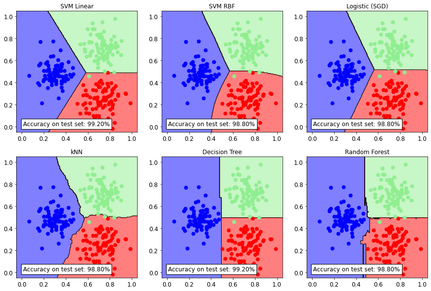
fig = CFigure(width=5 * len(clf_list) / 2, height=5 * 2)
for i, test_case in enumerate(clf_list):
clf = test_case.clf
xval_params = test_case.xval_parameters
print("\nEstimating the best training parameters of {:} ..."
"".format(test_case.clf_name))
best_params = clf.estimate_parameters(
dataset=tr, parameters=xval_params, splitter=xval_splitter,
metric='accuracy', perf_evaluator='xval')
print("The best parameters for '{:}' are: ".format(test_case.clf_name),
[(k, best_params[k]) for k in sorted(best_params)])
print("Training of {:} ...".format(test_case.clf_name))
clf.fit(tr.X, tr.Y)
# Predictions on test set and performance evaluation
y_pred = clf.predict(ts.X)
acc = metric.performance_score(y_true=ts.Y, y_pred=y_pred)
print("Classifier: {:}\tAccuracy: {:.2%}".format(test_case.clf_name, acc))
# Plot the decision function
from math import ceil
# Use `CFigure.subplot` to divide the figure in multiple subplots
fig.subplot(2, int(ceil(len(clf_list) / 2)), i + 1)
fig.sp.plot_decision_regions(clf, n_grid_points=200)
fig.sp.plot_ds(ts)
fig.sp.grid(grid_on=False)
fig.sp.title(test_case.clf_name)
fig.sp.text(0.01, 0.01, "Accuracy on test set: {:.2%}".format(acc),
bbox=dict(facecolor='white'))
fig.show()
Estimating the best training parameters of SVM Linear ...
The best parameters for 'SVM Linear' are:  [('C', 1)]
Training of SVM Linear ...
Classifier: SVM Linear  Accuracy: 99.20%

Estimating the best training parameters of SVM RBF ...
The best parameters for 'SVM RBF' are:  [('C', 1), ('kernel.gamma', 10)]
Training of SVM RBF ...
Classifier: SVM RBF     Accuracy: 98.80%

Estimating the best training parameters of Logistic (SGD) ...
The best parameters for 'Logistic (SGD)' are:  [('alpha', 1e-06)]
Training of Logistic (SGD) ...
Classifier: Logistic (SGD)      Accuracy: 98.80%

Estimating the best training parameters of kNN ...
The best parameters for 'kNN' are:  [('n_neighbors', 10)]
Training of kNN ...
Classifier: kNN Accuracy: 98.80%

Estimating the best training parameters of Decision Tree ...
The best parameters for 'Decision Tree' are:  [('max_depth', 3)]
Training of Decision Tree ...
Classifier: Decision Tree       Accuracy: 99.20%

Estimating the best training parameters of Random Forest ...
The best parameters for 'Random Forest' are:  [('n_estimators', 20)]
Training of Random Forest ...
Classifier: Random Forest       Accuracy: 98.80%