2.10. Using Foolbox attack classes within SecML
In this tutorial we will show how to execute Foolbox’s evasion attacks against machine learning models within SecML.
![]()
Warning
Requires installation of the pytorch and foolbox extra dependencies. See extra components for more information.
[1]:
%%capture --no-stderr --no-display
# NBVAL_IGNORE_OUTPUT

try:
  import secml
  import torch
  import foolbox
except ImportError:
  %pip install git+https://gitlab.com/secml/secml#egg=secml[pytorch,foolbox]
2.10.1. Training the model
The first part of the tutorial replicates the first part of 01-Training. We train a SVM RBF Multiclass classifier that will be used for crafting the attacks. We define here a simple 2D dataset which consists of 3 clusters of points, so that we can easily visualize the results.
[2]:
random_state = 999

n_features = 2  # Number of features
n_samples = 1100  # Number of samples
centers = [[-2, 0], [2, -2], [2, 2]]  # Centers of the clusters
cluster_std = 0.8  # Standard deviation of the clusters

from secml.data.loader import CDLRandomBlobs
dataset = CDLRandomBlobs(n_features=n_features,
                         centers=centers,
                         cluster_std=cluster_std,
                         n_samples=n_samples,
                         random_state=random_state).load()

n_tr = 1000  # Number of training set samples
n_ts = 100  # Number of test set samples

# Split in training and test
from secml.data.splitter import CTrainTestSplit
splitter = CTrainTestSplit(
    train_size=n_tr, test_size=n_ts, random_state=random_state)
tr, ts = splitter.split(dataset)

# Normalize the data
from secml.ml.features import CNormalizerMinMax
nmz = CNormalizerMinMax()
tr.X = nmz.fit_transform(tr.X)
ts.X = nmz.transform(ts.X)

# Metric to use for training and performance evaluation
from secml.ml.peval.metrics import CMetricAccuracy
metric = CMetricAccuracy()

# Creation of the multiclass classifier
from secml.ml.classifiers import CClassifierSVM
from secml.ml.classifiers.multiclass import CClassifierMulticlassOVA
from secml.ml.kernels import CKernelRBF
clf = CClassifierMulticlassOVA(CClassifierSVM, kernel=CKernelRBF())

# Set classifier's parameters
clf_params = {'C': 0.02, 'kernel.gamma': 50}
clf.set_params(clf_params)

# We can now fit the classifier
clf.fit(tr.X, tr.Y)

# Compute predictions on a test set
y_pred = clf.predict(ts.X)

# Evaluate the accuracy of the classifier
acc = metric.performance_score(y_true=ts.Y, y_pred=y_pred)

print("Accuracy on test set: {:.2%}".format(acc))
Accuracy on test set: 99.00%
2.10.2. Crafting the Adversarial Examples
Now that the model is trained, we can prepare the attacks against it. We are going to create adversarial examples using attacks from the Foolbox library.
Foolbox Rauber, Jonas and Brendel, Wieland and Bethge, Matthias Foolbox: A Python toolbox to benchmark the robustness of machine learning models. Reliable Machine Learning in the Wild Workshop, 34th International Conference on Machine Learning arXiv:1706.06083 [cs, stat]. 2017
For using the attacks from Foolbox in SecML, we can: * use the specific classes defined within SecML, which wrap directly a specific class of attack from Foolbox. These classes define the objective function for each attack. * For new attacks classes and attacks that don’t have an objective function, e.g., black-box attacks, we can use the generic class wrapper, which takes as input the Foolbox attack class with its initialization parameters.
We will use the following attacks:
with the wrappers in our library >* PGD >Madry A, Makelov A, Schmidt L, Tsipras D, Vladu A. Towards Deep Learning Models Resistant to Adversarial Attacks. >arXiv:1706.06083 [cs, stat] [Internet]. 2017
CW >Carlini N, Wagner D. Towards Evaluating the Robustness of Neural Networks. >arXiv:1608.04644 [cs] [Internet]. 2016
with the generic wrapper > * Salt-and-Pepper Wikipedia, Salt-and-pepper noise.
We can specify the starting point for the attacks. The selected point belongs to the class 1, which is in the lower right-corner of the 2D plane. Finally, we bound the features in the interval ‘[0, 1]’.
[3]:
x0, y0 = ts[1, :].X, ts[1, :].Y  # Initial sample
lb, ub = 0.0, 1.0  # Bounds of the attack space
2.10.2.1. Projected Gradient Descent (L2)
The first attack we are using against our classifier is the Projected Gradient Descent algoritmh with a L2 perturbation, which is wrapped with the SecML class CFoolboxPGDL2.
Projected Gradient Descent is a technique that finds an adversarial example that satisfies a norm constraint.
Here we choose a maximum perturbation of 0.2 from the initial point and we run an error-generic attack for 100 steps.
[4]:
steps = 100  # Number of iterations
epsilon = 0.2  # Maximum perturbation
y_target = None  # None if `error-generic`, the label of the target class for `error-specific`

from secml.adv.attacks.evasion import CFoolboxPGDL2
pgd_attack = CFoolboxPGDL2(clf, y_target,
                           lb=lb, ub=ub,
                           epsilons=epsilon,
                           abs_stepsize=0.01,
                           steps=steps,
                           random_start=False)
y_pred, _, adv_ds_pgd, _ = pgd_attack.run(x0, y0)

print("Original x0 label: ", y0.item())
print("Adversarial example label (PGD-L2): ", y_pred.item())

print("Number of classifier function evaluations: {:}"
      "".format(pgd_attack.f_eval))
print("Number of classifier gradient evaluations: {:}"
      "".format(pgd_attack.grad_eval))
Original x0 label:  1
Adversarial example label (PGD-L2):  2
Number of classifier function evaluations: 101
Number of classifier gradient evaluations: 100
As we see, the point has been wrongly classified by our model, exactly as we wanted.
We report the number of function evaluations and gradient evaluations that represent respectively how many times the methods for predictions and gradient are executed during the attack. The corresponding values depends on the number of steps the attack performs and on how the attack algorithm is defined.
We can also visualize the path that adversarial example took along the iterations, together with the objective function of the attack.
[5]:
from secml.figure import CFigure
# Only required for visualization in notebooks
%matplotlib inline

fig = CFigure(width=10, height=8, markersize=12)

# Replicate the `l2` constraint used by the attack for visualization
from secml.optim.constraints import CConstraintL2
constraint = CConstraintL2(center=x0, radius=epsilon)
# Plot the attack objective function
fig.sp.plot_fun(pgd_attack.objective_function, plot_levels=False,
                    multipoint=True, n_grid_points=200)
# Plot the decision boundaries of the classifier
fig.sp.plot_decision_regions(clf, plot_background=False, n_grid_points=200)

# Construct an array with the original point and the adversarial example
adv_path_pgd = x0.append(adv_ds_pgd.X, axis=0)

# Function for plotting the optimization sequence
fig.sp.plot_path(pgd_attack.x_seq)

# Function for plotting a constraint
fig.sp.plot_constraint(constraint)

fig.sp.title(pgd_attack.class_type)

fig.show()
fig.sp.grid(grid_on=False)

print("Initial point: {}".format(adv_path_pgd[0, :]))
print("Adversarial point: {}".format(adv_path_pgd[1, :]))
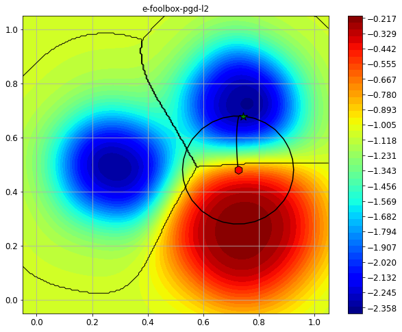
Initial point: CArray([[0.724797 0.479851]])
Adversarial point: CArray([[0.743075 0.679014]])
We can see how the initial point (red hexagon) has been perturbed in the feature space, and that our model classifies the final point as belonging to another class (green star).
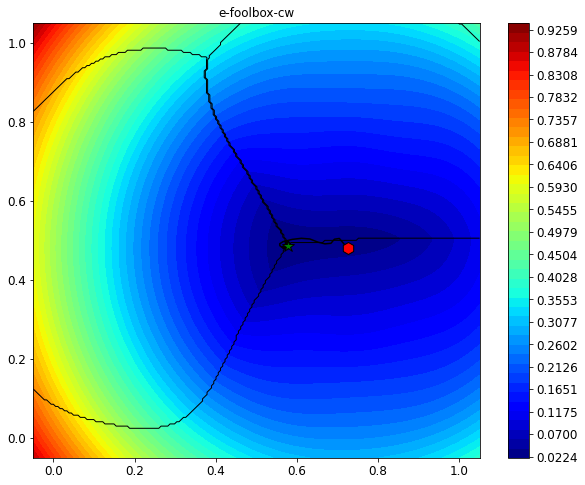
2.10.2.2. Carlini-Wagner Attack
The next attack we are showing is the Carlini & Wagner L2 attack. Carlini & Wagner attacks aim to find the smallest possible adversarial perturbation that causes a misclassification with a given confidence from the classifier.
This time we will run a targeted attack, sending the point to the leftmost decision region (y = 0).
[6]:
y_target = 0  # target class
stepsize = 0.05
steps = 100

from secml.adv.attacks.evasion import CFoolboxL2CarliniWagner
cw_attack = CFoolboxL2CarliniWagner(clf, y_target,
                                    lb=lb, ub=ub,
                                    steps=steps,
                                    binary_search_steps=9,
                                    stepsize=stepsize,
                                    abort_early=False)
y_pred, _, adv_ds_cw, _ = cw_attack.run(x0, y0)

print("Original x0 label: ", y0.item())
print("Adversarial example label (CW-L2): ", y_pred.item())

print("Number of classifier function evaluations: {:}"
      "".format(cw_attack.f_eval))
print("Number of classifier gradient evaluations: {:}"
      "".format(cw_attack.grad_eval))

from secml.figure import CFigure

# Only required for visualization in notebooks
%matplotlib inline

fig = CFigure(width=10, height=8, markersize=12)

# Plot the attack objective function
fig.sp.plot_fun(cw_attack.objective_function, plot_levels=False,
                    multipoint=True, n_grid_points=200)
# Plot the decision boundaries of the classifier
fig.sp.plot_decision_regions(clf, plot_background=False, n_grid_points=200)

# Construct an array with the original point and the adversarial example
adv_path_cw = x0.append(adv_ds_cw.X, axis=0)

# Function for plotting the optimization sequence
fig.sp.plot_path(cw_attack.x_seq)

fig.sp.title(cw_attack.class_type)

fig.show()
fig.sp.grid(grid_on=False)

print("Initial point: {}".format(adv_path_cw[0, :]))
print("Adversarial point: {}".format(adv_path_cw[1, :]))
Original x0 label:  1
Adversarial example label (CW-L2):  0
Number of classifier function evaluations: 901
Number of classifier gradient evaluations: 900
Initial point: CArray([[0.724797 0.479851]])
Adversarial point: CArray([[0.575826 0.4913  ]])
2.10.3. Using the generic wrapper
If we want to execute a Foolbox attack that is not directly implemented in SecML, we can use the generic wrapper. Here we show how to use the generic wrapper to execute on SecML the Salt-and-Pepper noise attack implemented in Foolbox.
Salt and Pepper noise (usually applied to images), perturbs an increasing number of feature values bringing them to the limits of the feature space, until the sample is misclassified.
It is indeed a “black-box” attack, i.e., the gradient of the classifier is not evaluated while performing the attack.
[7]:
# set the random state of torch in order to ensure the same
# result, as Salt and Pepper attack exploits randomness
import torch
torch.manual_seed(0)

y_target = None

from secml.adv.attacks.evasion import CAttackEvasionFoolbox
from foolbox.attacks.saltandpepper import SaltAndPepperNoiseAttack

# create the attack
sp_attack = CAttackEvasionFoolbox(clf, y_target,
                                  lb=lb, ub=ub,
                                  fb_attack_class=SaltAndPepperNoiseAttack,
                                  epsilons=None,
                                  steps=15,
                                  across_channels=False)

y_pred, _, adv_ds_sp, _ = sp_attack.run(x0, y0)

print("Original x0 label: ", y0.item())
print("Adversarial example label (Salt & Pepper): ", y_pred.item())

print("Number of classifier function evaluations: {:}"
      "".format(sp_attack.f_eval))
print("Number of classifier gradient evaluations: {:}"
      "".format(sp_attack.grad_eval))

from secml.figure import CFigure

# Only required for visualization in notebooks
%matplotlib inline

fig = CFigure(width=16, height=8, markersize=12)

# Plot the decision boundaries of the classifier
fig.subplot(1,2,1)
fig.sp.plot_decision_regions(clf, plot_background=True,
                             n_grid_points=200)

# Function for plotting the optimization sequence
fig.sp.plot_path(sp_attack.x_seq, path_color='green')
fig.sp.scatter(adv_ds_sp.X[0, 0], adv_ds_sp.X[0, 1])
fig.sp.text(x=adv_ds_sp.X[0, 0].item() + 0.03,
            y=adv_ds_sp.X[0, 1].item() - 0.1,
            s="adversarial point\nreturned by the attack",
            backgroundcolor='white')

fig.sp.title(sp_attack.class_type)

# classifier's output along the path
true_labels=torch.empty(sp_attack.x_seq.shape[0], dtype=torch.long).fill_(y0.item())
preds, scores = clf.predict(sp_attack.x_seq, return_decision_function=True)
# norm of perturbation along the path
path_distance = (sp_attack.x_seq - x0).norm_2d(order=2, axis=1).ravel()

best_step = (sp_attack.x_seq - adv_ds_sp.X).abs().sum(axis=-1)
best_step = best_step.argmin()

fig.subplot(1,2,2)
fig.sp.title("Classifier's outputs along the adversarial path")
fig.sp.plot(preds, color='r',
            label='output class (y_true = {})'.format(y0.item()))
fig.sp.plot(path_distance, color='b', label='norm of perturbation')
fig.sp.scatter(best_step, preds[best_step], c='r')
fig.sp.scatter(best_step, path_distance[best_step], c='b')
fig.sp.legend()
fig.show()
fig.sp.grid(grid_on=False)

print("Initial point: {}".format(x0))
print("Adversarial point: {}".format(adv_ds_sp.X))
Original x0 label:  1
Adversarial example label (Salt & Pepper):  2
Number of classifier function evaluations: 17
Number of classifier gradient evaluations: 0
Initial point: CArray([[0.724797 0.479851]])
Adversarial point: CArray([[0.724797 1.      ]])
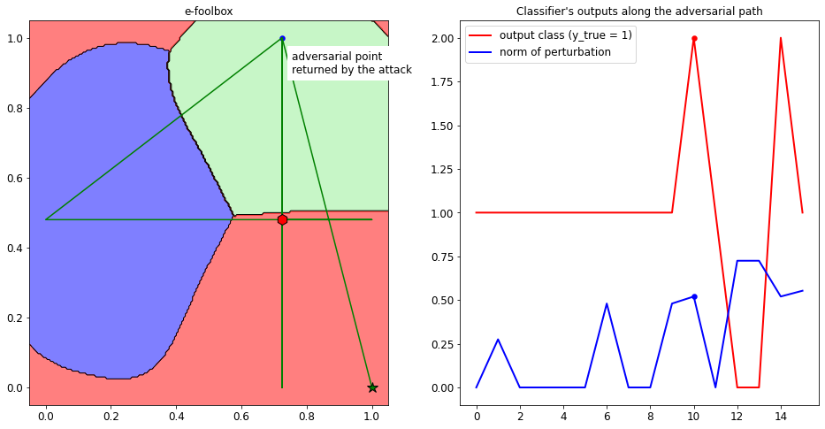
We can see that the number of gradient evaluations is zero, as expected. The attack is perturbing one feature at a time, by bringing them to the maximum or minimum value, until the sample is misclassified. From the plot in the right side, we can see that the best point returned (marked with the dots) is the one that causes a misclassification with the minimum L2 distance from the clean input x0.
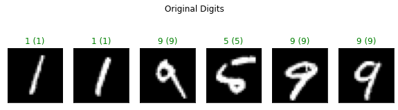
2.10.4. Crafting Adversarial Example on the MNIST Dataset
We can now use the Foolbox attacks to create adversarial examples against a convolutional neural network trained on the MNIST dataset.
We first load the MNIST dataset, and the pre-trained model from the model zoo.
[8]:
n_ts = 1000  # number of testing set samples

# Load MNIST Dataset
from secml.data.loader import CDataLoaderMNIST
digits = (1, 5, 9)
loader = CDataLoaderMNIST()
tr = loader.load('training', digits=digits)
ts = loader.load('testing', digits=digits, num_samples=n_ts)

# Normalize the data
tr.X /= 255
ts.X /= 255
[9]:
%%capture --no-stderr --no-display
# NBVAL_IGNORE_OUTPUT

# Load pre-trained model
from secml.model_zoo import load_model
clf = load_model('mnist159-cnn')

#Select dataset for the attack
attack_ds = ts[:6, :]
We can use this model to classify the digits and show the accuracy.
[10]:
labels = clf.predict(ts.X, return_decision_function=False)

from secml.ml.peval.metrics import CMetric
metric = CMetric.create('accuracy')
acc = metric.performance_score(ts.Y, labels)

print("Model Accuracy: {}".format(acc))
Model Accuracy: 0.997
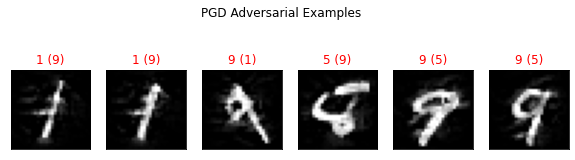
Now we can craft adversarial example using the attacks previously introduced and display them as images, to see the results obtained by different attacks.
[11]:
y_target = None
steps = 100
epsilon = 2.6
pgd_attack = CFoolboxPGDL2(clf, y_target,
                           lb=lb, ub=ub,
                           epsilons=epsilon,
                           abs_stepsize=0.1,
                           steps=steps,
                           random_start=False)

print("PGD-L2 Attack started...")
y_pred_pgd, _, adv_ds_pgd, _ = pgd_attack.run(attack_ds.X, attack_ds.Y)
print("PGD-L2 Attack complete!")
PGD-L2 Attack started...
PGD-L2 Attack complete!
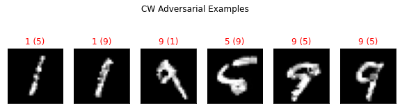
[12]:
y_target = None
steps = 100
stepsize= 0.03
cw_attack = CFoolboxL2CarliniWagner(clf, y_target,
                                    lb=lb, ub=ub,
                                    steps=steps,
                                    binary_search_steps=9,
                                    stepsize=stepsize,
                                    abort_early=False)

print("CW-L2 Attack started...")
y_pred_cw, _, adv_ds_cw, _ = cw_attack.run(attack_ds.X, attack_ds.Y)
print("CW-L2 Attack complete!")
CW-L2 Attack started...
CW-L2 Attack complete!
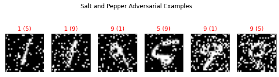
[13]:
y_target = None
sp_attack = CAttackEvasionFoolbox(clf, y_target,
                                  lb=lb, ub=ub,
                                  fb_attack_class=SaltAndPepperNoiseAttack,
                                  epsilons = None)

print("Salt and Pepper Attack started...")
y_pred_sp, _, adv_ds_sp, _ = sp_attack.run(attack_ds.X, attack_ds.Y)
print("Salt and Pepper Attack complete!")
Salt and Pepper Attack started...
Salt and Pepper Attack complete!
Finally, we display both the original and the adversarial digits along with their labels.
[14]:
from secml.figure import CFigure
# Only required for visualization in notebooks
%matplotlib inline

# Function to plot the MNIST dataset
def show_digits(samples, preds, labels, digs, title):
    samples = samples.atleast_2d()
    n_display = samples.shape[0]
    fig = CFigure(width=10, height=3)
    fig.title("{}".format(title))
    for idx in range(n_display):
        fig.subplot(1, n_display, idx+1)
        fig.sp.xticks([])
        fig.sp.yticks([])
        fig.sp.imshow(samples[idx, :].reshape((28, 28)), cmap='gray')
        fig.sp.title("{} ({})".format(digits[labels[idx].item()], digs[preds[idx].item()]),
                     color=("green" if labels[idx].item()==preds[idx].item() else "red"))
    fig.show()

show_digits(attack_ds.X[:, :], clf.predict(attack_ds.X[:, :]), attack_ds.Y[:, :], digits, "Original Digits")
show_digits(adv_ds_pgd.X[:, :], clf.predict(adv_ds_pgd.X[:, :]), adv_ds_pgd.Y[:, :], digits, "PGD Adversarial Examples")
show_digits(adv_ds_cw.X[:, :], clf.predict(adv_ds_cw.X[:, :]), adv_ds_cw.Y[:, :], digits, "CW Adversarial Examples")
show_digits(adv_ds_sp.X[:, :], clf.predict(adv_ds_sp.X[:, :]), adv_ds_sp.Y[:, :], digits, "Salt and Pepper Adversarial Examples")